Analyzing the NYC Subway Dataset
Section I: Introduction
Project Topics: Data Wrangling, Statistics, Machine Learning, and Effective Visualizations
This is the second project of the Udacity Data Analyst Nanodegree. In it we analyze the NYC Subway Dataset to find out if more people take the subway when it's raining than when it is not. It consists of two parts. Part 1 of the project is to answer Problem sets 2, 3, and 4 of the course Intro to Data Science on Udacity. This course gives an introduction to many tools necessary for aspiring data scientists to know, like exploratory analysis, data wrangling, interacting with large datasets through sql, applying statistical tests, using machine learning for predicting outcomes, and visualizing data. Part 2 is a reflection of how the problem sets were solved and why specific statistical tests might have been chosen. Combining these two parts I will try to guide you through my thought process as I was solving the problem sets.
The NYC Subway Dataset
The NYC Subway dataset is a huge dataset consisting of over 100000 rows and about 22 columns of data. The dataset has the number of entries and exits registered by specific subway units at specific dates and at specific times a day. Furthermore, it has weather related information at these specific timestamps, like whether or not it was raining, whether or not it was foggy, and many more. Below is a list of all the columns, and for more information on what these specific parameters are see this document.
import pandas as pd
turnstile_weatherdata = pd.read_csv("./data/turnstile_data_master_with_weather.csv",
                                    sep=",")

# turnstile_weatherdata.take(1)
for c in turnstile_weatherdata.columns.values[1:]:
    print "%s," % c,
Section II: References
Throughout this project and the Introduction to Data Science course, I used a number of resources, besides the course material, to help me answer some of the questions. Here you'll find a list of these references, which might benefit you if you're ever in a situation where you need to analyze a large dataset and want to do some statistical tests on it. Furthermore, reading some of these links might actually give you ideas for other things you could try on your dataset.
Visualizations and Inspiration
- Mapping NYC Taxi Data
- Basemap
- FlowingData
- Working with Maps in Python
- More Working with Maps in Python
Understanding the Statistical Tests
- Mann-Whitney U Test
- Hypethesis Testing
- Some more Hypothesis Testing
- Welch's T Test
- Shapiro Wilks Test (the accepted answer)
Statistical Tests in Python
Section III: Independent and dependent variables, Statistical Test, and Descriptive Statistics
Independent and dependent variables
In this project, the role of the dependent variable goes to the number of people taking the subway, which in this dataset is somewhat represented by the ENTRIESn_hourly column. The independent variables are the variables we chose to use as predictor variables. In the Linear Regression section I'll get deeper into the choice of predictor/independent variables and why they were chosen.
Null- and Alternative Hypothesis
The NYC Subway Dataset is huge and one could theoretically analyze it for many different things. However, for this analysis, we want to find out if more or less people are using the subway when it is raining. Stated differently we want to analyse if there is a statistical significant difference between the observations of subway users from population X and Y, where X is when it is raining and Y is when it isn't. The null- and alternative hypothesis are:
- Null hypothesis: There is no significant difference in the amount of observed subway users when it is and when it isn't raining:
- Alternative hypothesis: There is a significant difference in the amount of subway users when it is raining compared to when it isn't:
Statistical Test
In previous projects we have either been using a z-test or t-test, but for these statistical tests to be viable, we must be able to assume that the data is normally distributed. In Problem Set 3.1 of the Introduction to Data Science we produced two histograms illustrating how the ENTRIESn_hourly was distributed when was and wasn't raining. This figure is shown below and from it we can see that this data isn't normally distributed.
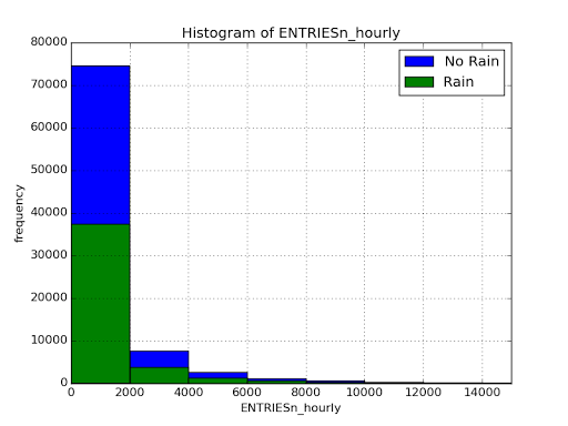 This is of course only one way to test for the normality of the data. We can also run a Shapiro Wilks test on the data. This gives us a $ W = 0.475 $ and $ p = 0.0 < 0.05 = p_{critical} $ meaning we can reject the null hypothesis of this data being normally distributed. However, as is explained and shown very well in the link to the Shapiro Wilks Test, this normality test can fail quite often and therefore looking at the histograms might be a better way to ensure that the data is normally or non-normally distributed.
Because the assumption of normallity is rejected we will be using the one-tailed Mann-Whitney U Test with a $ p_{critical} = 0.05 $.
Statistical Test Results
Running the Mann-Whitney U Test on the data is done in problem set 3.3 in the Introduction to Data Science course. The two inputs to the Mann-Whitney U Test are the ENTRIESn_hourly for when it rains and when it doesn't. The results of this test are:
| Statistic | Rain | No Rain |
|---|---|---|
| $\bar{x}_{ENTRIESn\_hourly}$ | 1105.4463767458733 | 1090.278780151855 |
and the U and p values returned from the scipy.stats.mannwhitneyu test were:
$$ (U, p) \simeq (1924409167.0,\, 0.025) $$The scipy.stats.mannwhitneyu test returns the result of a one-tailed test, but converting this to a two tailed is a matter of multiplying by two. So our $ p = 0.024999912793489721 \simeq 0.025 $ for a one-tailed test is the same as a $ p = 0.04999982558697944 \simeq 0.05 $ for a two-tailed test. With a $ p_{critical} = 0.05 $ we see that $ p \simeq 0.05 < 0.05 = p_{critical} $ meaning we can reject the null hypothesis. The significance of this test is that it shows that there are not the same amount of people using the subway when it is and when it isn't raining. From the reported means we can also see that the the distribution for which it was raining is statistically greater than when it isn't. We must however notice that the U value returned from the scipy.stats.mannwhitneyu test is very large. Since smaller U values indicate greater deviations from the null hypothesis, this large U value indicates a very small deviation from the null hypothesis.
Section IV: Linear Regression, Predicting the Number of Subway Users
To try and predict the number of ENTRIESn_houly I chose to use the Statsmodels ordinary least squares linear regressor. OLS was chosen because I found it to give better and more consistent results. The input variables for the OLS model were rain, precipi, meantempi, maxpressurei, minpressurei, maxdewpti, fog, meanwindspdi, weekday, Hour, rush_hour, UNIT The reason behind the inputs are different as some were chosen because random testing showed them to have an effect on the predictability of the model, whilst others were chosen because I believed that these features had an effect on how well a model could predict.
- Test chosen features: rain, meanwindspdi, precipi, meantempi, maxpressurei, minpressurei, maxdwpti, fog
- Reason chosen features: weekday, hour, rush_hour, UNIT, warm, cold, dry, moist, humid, windy
The test chosen features were found when testing the predictability and adding features to try and find some improvement. Some features, like maxpressurei, minpressurei, maxdwpti were added at random and were kept because they turned out to increase predictability. Other features like rain, meanwindspdi, precipi, and meantempi were added because I had the idea that rain, wind and temperature would have an effect on how many people would use the subway. Adding features based on "raw" data works well to some degree. However, this is not always the best way to increase predictability of a model. Oftentimes one can increase the predictability vastly by either creating dummy variables, as was done with the UNIT feature, or creating boolean features as was done for the weekday, rush_hour, warm, cold, dry, moist, humid, windy features. The dummy feature is a simple way to create numeric features from non-numeric data, i.e. going from categorical data like the UNIT column which consists of names of the units which record the ENTRIESn_hourly, to $N$ columns, where $N$ is the number of unique units. The boolean features were created because I believed that there was a greater amount of people using the subway during the weekdays than during the weekends, and also a greater amount of people using the subway in what I call rush_hour, which is a time interval from 10.00 (10am) to 22.00 (10pm). Furthermore all the weather related boolean features were created because I assumed that more people would use the subway during extreme(r) weather conditions (this actually increased my $R^2$ from 0.47 to about 0.5).
By using these features in the OLS the weights for the non-dummy features were:
| Feature | Weight |
|---|---|
| const | 14397.602439 |
| rain | -263.684249 |
| warm | -55.935904 |
| moist | 388.166843 |
| dry | 132.037170 |
| humid | -492.742290 |
| windy | -238.417431 |
| cold | -151.507613 |
| precipi | 209.676586 |
| maxpressurei | -653.533281 |
| minpressurei | 265.309983 |
| fog | 65.282306 |
| meanwindspdi | 26.384006 |
| weekday | 522.478287 |
| Hour | 24.224710 |
| meantempi | -31.054565 |
| maxdewpti | -5.279691 |
| rush_hour | 696.724312 |
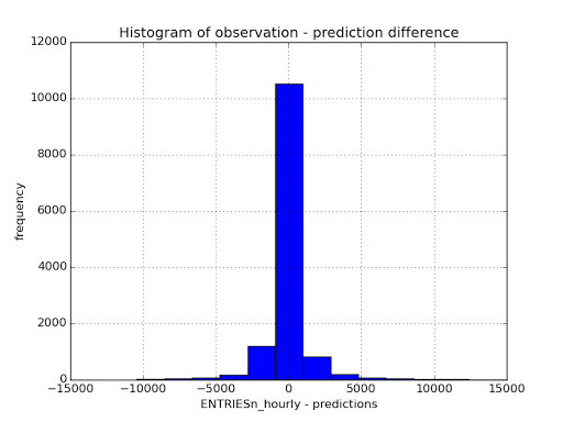
and the coefficient of determination returned was $R^2 = 0.499235384485 \simeq 0.5$. The point of the $R^2$ is to give an idea of how well the model fits the data. Because we have a coefficient of determination of about $0.5$ we can say that the model, using the current features explains $50\%$ of the variability of the number of subway users. From my tests on the data set it seemed very hard to increase the coefficient of determination above $0.5$ and therefore I believe that this model fits the data to the best of its ability. Meaning that the model is somewhat succesful at predicting the number of subway users, but that it might be a too simple model. Below we also see a histogram showing the difference between the observed ENTRIESn_hourly and the predicted. The plot shows that the
Section V: Conclusion
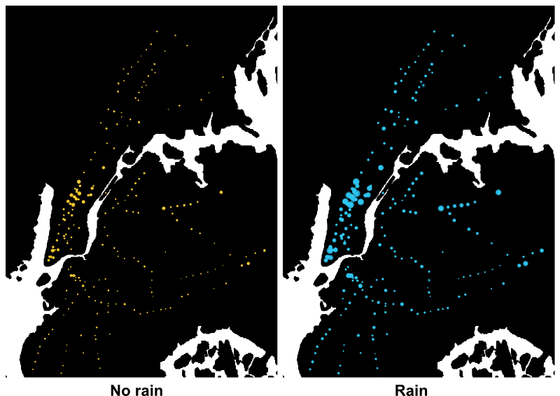
We have throughout the analysis of the NYC subway dataset tried to find out if there are more people riding the NYC subway when it is raining then when it isn't, and also tried to build a statistical machine learning model to predict the number of subway users based on some features of our own chosing/making. I believe that the best illustration of whether or not more people ride the NYC subway when it is raining is actually the first figure I show, which was the first analysis I did on the data. On this figure we see the normalized NYC subway riders per station/unit grouped into raining and not raining plotted on a map of NY. I think it quite clearly shows that more people use the NYC subway when it is raining than when it isn't. From this analysis there is also another result, which might convey a more statistical way of indicating a greater ridership when it is raing than when it isn't. This is the result from the statistical test which showed that the null hypothesis, of the number of subway users being the same when it was raining and when it wasn't, could be rejected. However, we also see from the OLS that the weight for the rain feature is negative! This could mean that the rain feature has a negative effect on the number of subway users, or it could be an effect of multicollinearity, i.e. that some of my features are highly linearly related. This is very likely since e.g. temperature, humidity, pressure and wind are all highly correlated.
Section VI: Reflection
As a whole, I'm amazed at how much data is available if you just look for it. This dataset inspired me to look at other datasets, and I found many interesting public dataset, like the NYC taxi data. However there are some things about this particular dataset which bothered me, and if different might have resulted in a better model. Some shortcomings of the dataset are the lack of consistent measurements. We have measurements of ENTREISn_hourly at various hours of the day, but there is no continuous timeseries of measurements. I am well aware of the fact that the data for ENTRIESn_hourly is inherently discrete, but the lack of consistent measurements bothered me. Some things I could've done differently, was to visualize the data to try and find some patterns in the data. This could've been done through clustering or grouping the data. Furthermore, my analysis was done using a linear regression model, but I strongly believe that the data is non-linear and that a non-linear regressor could've performed better.